Jianfeng Xiang | Blogs | FlexGEMM: A Cross-Platform Backend for High-Performance Sparse Convolutions

Preface

Doing research is often an art of maximizing the value of limited resources.

During the development of the 3D generative model Trellis.2, I increasingly felt constrained by the hardware environment. As the resolution of sparse convolutions increased, so did memory usage and computation cost. However, the number of high-performance NVIDIA GPUs available for training was limited, while many more advanced AMD GPUs remained almost unusable due to compatibility issues. At that time, mainstream sparse convolution libraries (such as spconv [1] and torchsparse [2]) were deeply tied to the CUDA ecosystem—essentially unusable on AMD GPUs. In other words, despite having accessible compute power, I was “locked out” by software ecosystem barriers. For research, this situation was extremely frustrating.

It was in this context that I realized the need for FlexGEMM—a general backend that could both squeeze the maximum performance out of sparse computation and enable smooth switching across different GPU platforms.

Building such a truly cross-platform backend was far from easy. Initially, I tried porting existing sparse convolution libraries, but those codebases were heavily dependent on CUDA kernels and PTX assembly, deeply bound to the NVIDIA ecosystem, making migration to AMD nearly impossible.

Things changed when I came across Triton [3]. Triton is a GPU programming language developed by OpenAI that abstracts GPU kernel programming with a Python-like syntax, allowing me to directly control computation parallelism and memory access at a higher level. More importantly, Triton’s backend not only supports CUDA but has also been steadily improving support for ROCm (AMD’s GPU software stack). This meant I could finally drive GPUs across platforms with the same codebase.

In research practice, this is critical: I no longer need to maintain two separate implementations for different hardware, nor do I have to worry about valuable compute sitting idle. Triton’s unified programming paradigm became the cornerstone for building FlexGEMM.

Beyond that, Triton comes with built-in optimization strategies tailored for different hardware architectures—for example, efficient shared memory usage, vectorized global memory access, hardware-accelerated matrix multiplication, and pipelining to hide cache latency. Traditionally, these techniques required deep, platform-specific expertise (like handling Tensor Cores), which meant high learning costs and poor code portability. With Triton, kernel developers can simply write one piece of code, and the compiler will extract near-optimal performance across platforms. As a result, kernels written in Triton not only accelerate current hardware but also remain future-proof, adapting to new GPUs with minimal new code.

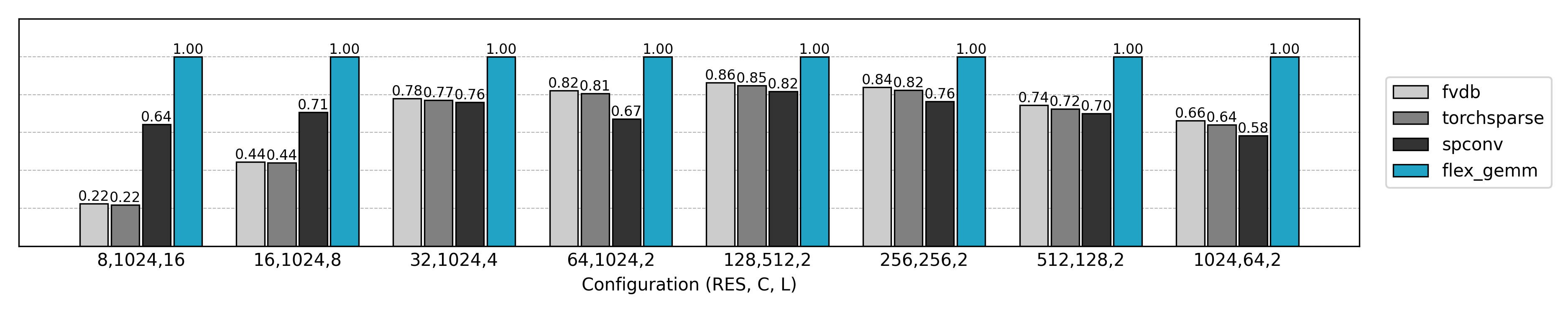
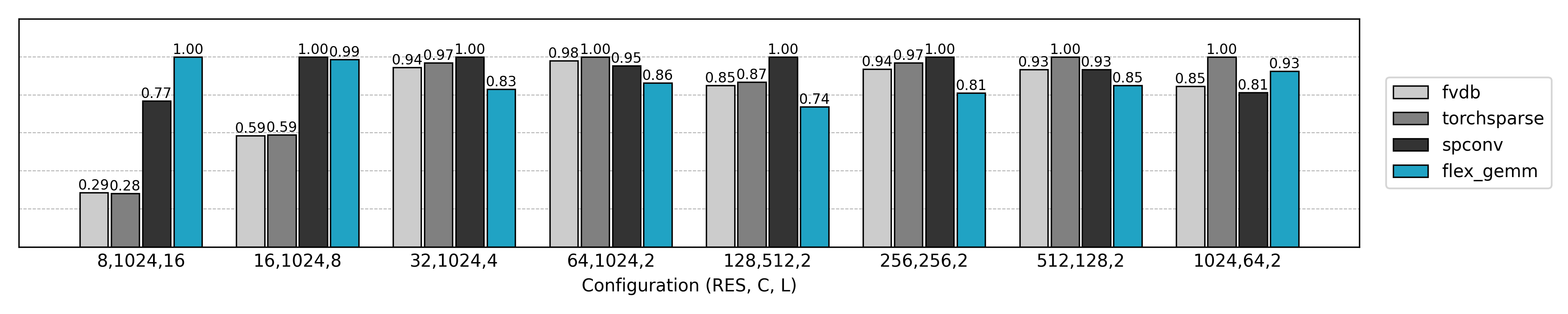
Thanks to Triton’s cross-platform capabilities and flexible optimizations, FlexGEMM performs exceptionally well in real 3D sparse convolution workloads: compared to mainstream libraries, it achieves up to ~2× acceleration in efficient numerical formats such as FP16/TF32. Even better, it runs seamlessly on both NVIDIA and AMD GPUs—without maintaining separate codebases. In other words, FlexGEMM not only unleashes compute power but also provides true flexibility and scalability for research—ready for today’s hardware and tomorrow’s GPUs alike.

Training speed comparison under FP16 precision

Inference speed comparison under FP16 precision

Training speed comparison under TF32 precision

Inference speed comparison under TF32 precision

Training speed comparison under FP32 precision

Inference speed comparison under FP32 precision

Starting from Naive Convolutions

Before diving into the implementation of FlexGEMM, let’s begin with the most straightforward way to implement sparse convolutions. Readers familiar with classic convolutions may already know that a convolution operation can be equivalently transformed into a matrix multiplication: the first operand is the feature map expanded via im2col (flattening local neighborhoods into columns), and the second operand is the convolution kernel weights. In other words, a convolution is essentially a large-scale GEMM (General Matrix Multiplication):

import torch
import torch.nn.functional as F

# Parameter definitions
B, Ci, Co, K, H, W = 1, 3, 4, 3, 5, 5   # batch, in_channels, out_channels, kernel, height, width

# Input: [B, Ci, H, W]
x = torch.randn(B, Ci, H, W)

# Convolution kernel: [Co, Ci, K, K]
weight = torch.randn(Co, Ci, K, K)

# Use im2col to unfold input neighborhoods
# unfold output: [B, Ci*K*K, L], where L = H*W (number of positions after padding)
cols = F.unfold(x, kernel_size=K, padding=K//2)   # [B, Ci*K*K, H*W]

# Transpose to [B, L, Ci*K*K]
cols = cols.transpose(1, 2)   # [B, H*W, Ci*K*K]

# Flatten weights: [Co, Ci*K*K]
w = weight.view(Co, -1)       # [Co, Ci*K*K]

# GEMM: [B, L, Ci*K*K] @ [Ci*K*K, Co] = [B, L, Co]
out = cols @ w.T              # [B, H*W, Co]

# Restore as feature map: [B, Co, H, W]
out = out.transpose(1, 2).view(B, Co, H, W)

This algorithm is called Explicit GEMM, meaning explicit general matrix multiplication. By explicitly constructing the flattened input feature map, convolution can be performed with a single matrix multiplication.

For sparse convolutions, we can adopt a similar workflow to first build a naive implementation. The main challenge, however, lies in how to efficiently fetch local neighborhoods of sparse input features. Unlike dense tensors, the neighbors of sparse tensors cannot be obtained via simple slicing or algebraic indexing, but instead require additional data structures and search procedures.

Fetching Local Neighborhoods

There are many algorithms and data structures for retrieving local neighborhoods of sparse data. For example, O-CNN [4] accelerates spatial queries with octrees, while fVDB [5] leverages VDB structures for efficient indexing. In FlexGEMM, I opted for the most straightforward approach: hash table–based neighborhood queries.

Hash Tables on GPU

Here, I followed Nosferalatu’s minimal CUDA hash table implementation [6], which uses open addressing with linear probing, along with atomic operations to ensure concurrency safety. Compared to complex data structures requiring locks, this approach is much better suited for GPU parallelism. Below is the core insertion and lookup logic:

__forceinline__ __device__ void linear_probing_insert(
    uint32_t* hashmap,
    const uint32_t keys,
    const uint32_t values,
    const int64_t N
) {
    uint32_t slot = hash(keys, N);
    while (true) {
        uint32_t prev = atomicCAS(&hashmap[slot], K_EMPTY, keys);
        if (prev == K_EMPTY || prev == keys) {
            hashmap[slot + N] = values;
            return;
        }
        slot = (slot + 1) % N;
    }
}

__forceinline__ __device__ uint32_t linear_probing_lookup(
    const uint32_t* hashmap,
    const uint32_t keys,
    const int64_t N
) {
    uint32_t slot = hash(keys, N);
    while (true) {
        uint32_t prev = hashmap[slot];
        if (prev == K_EMPTY) {
            return K_EMPTY;
        }
        if (prev == keys) {
            return hashmap[slot + N];
        }
        slot = (slot + 1) % N;
    }
}

Here, the hashmap is actually composed of two parts: the first half stores keys, and the second half stores the corresponding values. Hence the array size is 2N.

hashmap[slot] stores the key
hashmap[slot + N] stores the value

Insert

Compute the initial slot using hash(keys, N).
Use atomicCAS (atomic compare-and-swap) to attempt writing the key:
- If the slot is empty (K_EMPTY), write the key and store the value.
- If the slot already contains the same key, update the value.
- Otherwise, a collision occurs—continue probing with (slot + 1) % N.

Lookup

Hash to locate the slot.
If the slot is empty, the key doesn’t exist.
If the key matches, return the corresponding value.
Otherwise, keep probing linearly until the target is found or an empty slot is reached.

This approach is simple and efficient, especially for large-scale parallel queries on GPUs. While linear probing may lead to long search chains in the worst case, under a reasonable load factor it maintains high throughput.

For the hash function, I reused the murmur3 hash function from the reference implementation:

__forceinline__ __device__ uint32_t hash(uint32_t k, uint32_t N) {
    k ^= k >> 16;
    k *= 0x85ebca6b;
    k ^= k >> 13;
    k *= 0xc2b2ae35;
    k ^= k >> 16;
    return k % N;
}

Inserting Sparse Tensor Coordinates

The above implementation works for uint32 scalar keys. Handling 3D (or 4D) sparse tensor coordinates is straightforward: serialize them into a unique uint32 key. The CUDA kernel below shows how to insert sparse tensor coordinates [b, x, y, z] into the hash table:

/**
 * Insert 3D coordinates into the hashmap using index as value
 * 
 * @param N         number of elements in the hashmap
 * @param M         number of 3d coordinates
 * @param W         the number of width dimensions
 * @param H         the number of height dimensions
 * @param D         the number of depth dimensions
 * @param hashmap   [2N] uint32 tensor containing the hashmap (key-value pairs)
 * @param coords    [M, 4] int32 tensor containing the keys to be inserted
 */
__global__ void hashmap_insert_3d_idx_as_val_cuda_kernel(
    const uint32_t N,
    const uint32_t M,
    const int W,
    const int H,
    const int D,
    uint32_t* __restrict__ hashmap,
    const int32_t* __restrict__ coords
) {
    uint32_t thread_id = blockIdx.x * blockDim.x + threadIdx.x;
    if (thread_id < M) {
        int4 coord = reinterpret_cast<const int4*>(coords)[thread_id];
        int b = coord.x;
        int x = coord.y;
        int y = coord.z;
        int z = coord.w;
        uint32_t key = static_cast<uint32_t>((((b * W + x) * H + y) * D + z));
        linear_probing_insert(hashmap, key, thread_id, N);
    }
}

Each thread in this kernel processes one element of the sparse tensor. To maximize memory bandwidth, the program uses 128-bit aligned memory loads to fetch the four coordinates [b, x, y, z] in one go. Then the coordinates are mapped to a globally unique integer ID via key = (((b * W + x) * H + y) * D + z).

Meanwhile, the hash table stores the thread_id as the value, which corresponds to the index of the point in the input coordinate array. This way, during neighborhood lookups, we can directly retrieve the sparse tensor index from the hash table and access the corresponding feature value.

Observant readers may have noticed that the key is defined as a uint32, meaning it can represent at most $2^{32}-1$ unique IDs. In the context of sparse tensors, this corresponds to roughly a 1024³ voxel grid with batch size 4. For most applications, this capacity is more than sufficient. If larger resolutions are required, the key type can be extended to uint64, allowing a larger integer space. However, this increases the cost of hashing and memory access, potentially reducing efficiency.

Querying Neighborhood Indices

After constructing the hash table of sparse tensor coordinates, the next step is to use it for fast convolutional neighborhood queries. Specifically, given a sparse point [b, x, y, z] and kernel size (Kw, Kh, Kd), we want to determine in constant time whether each neighbor exists and retrieve its index in the sparse tensor. The CUDA kernel below shows how to efficiently generate a submanifold convolution neighbor map based on the hash table:

Submanifold convolution (submconv) is a special form of sparse convolution. In standard sparse convolution, the kernel may activate new points in the neighborhood (expanding the active region). Submanifold convolution, however, requires the output active points to match the input, without introducing new nonzeros. This makes submconv ideal for stacking deep networks while preserving sparsity, and it is the most commonly used convolution type in current 3D generative tasks.

/**
 * Lookup sparse submanifold convolution neighbor map with hashmap
 * 
 * @param N         number of elements in the hashmap
 * @param M         number of 3d coordinates
 * @param W         the number of width dimensions
 * @param H         the number of height dimensions
 * @param D         the number of depth dimensions
 * @param V         the volume of the kernel
 * @param Kw        the number of width kernel dimensions
 * @param Kh        the number of height kernel dimensions
 * @param Kd        the number of depth kernel dimensions
 * @param Dw        the dilation of width
 * @param Dh        the dilation of height
 * @param Dd        the dilation of depth
 * @param hashmap   [2N] uint32 tensor containing the hashmap (key-value pairs)
 * @param coords    [M, 4] int32 tensor containing the keys to be looked up
 * @param neighbor [M, Kw * Kh * Kd] uint32 tensor containing the submanifold convolution neighbor map
 */
__global__ void hashmap_lookup_submanifold_conv_neighbour_map_cuda_kernel(
    const uint32_t N,
    const uint32_t M,
    const int W,
    const int H,
    const int D,
    const int V,
    const int Kw,
    const int Kh,
    const int Kd,
    const int Dw,
    const int Dh,
    const int Dd,
    const uint32_t* __restrict__  hashmap,
    const int32_t* __restrict__  coords,
    uint32_t* __restrict__ neighbor
) {
    int64_t thread_id = blockIdx.x * blockDim.x + threadIdx.x;
    int half_V = V / 2 + 1;
    uint32_t idx = thread_id / half_V;
    if (idx < M) {
        int4 coord = reinterpret_cast<const int4*>(coords)[idx];
        int b = coord.x;
        int x = coord.y - Kw / 2 * Dw;
        int y = coord.z - Kh / 2 * Dh;
        int z = coord.w - Kd / 2 * Dd;
        int KhKd = Kh * Kd;
        int v = thread_id % half_V;
        
        uint32_t value = K_EMPTY;
        if (v == half_V - 1) {
            value = idx;
        }
        else {
            int kx = x + v / KhKd * Dw;
            int ky = y + v / Kd % Kh * Dh;
            int kz = z + v % Kd * Dd;
            if (kx >= 0 && kx < W && ky >= 0 && ky < H && kz >= 0 && kz < D) {
                uint32_t key = static_cast<uint32_t>((((b * W + kx) * H + ky) * D + kz));
                value = linear_probing_lookup(hashmap, key, N);
                if (value != K_EMPTY) {;
                    neighbor[value * V + V - 1 - v] = idx;
                }
            }
        }
        neighbor[idx * V + v] = value;
    }
}

In this kernel, we build a neighbor index map for each sparse point. The map has shape [M, Kw * Kh * Kd], where M is the number of sparse points, and Kw, Kh, Kd are the kernel dimensions.

1. Thread assignment

Each thread corresponds to a query task for a sparse point at a specific kernel offset (idx, v):

idx is the index of the sparse point.
v is the index of the offset within the convolution kernel.

2. Compute kernel center offset

By shifting with Kw/2, Kh/2, Kd/2, the kernel is centered on the point: v=0 corresponds to the front-top-left corner, and v=V/2 corresponds to the center.

3. Boundary check

When translating the kernel to the input coordinates, ensure the location (kx, ky, kz) lies within [0, W) × [0, H) × [0, D). Otherwise, the neighbor is invalid.

4. Hash table lookup

Compute the unique integer key for valid coordinates (b, kx, ky, kz), then call linear_probing_lookup(hashmap, key, N).

If found, return the neighbor’s index in the sparse coordinate array.
If not found, mark as K_EMPTY.

5. Update neighbor map

Write the result into neighbor[idx * V + v]. The kernel center (v == half_V - 1) corresponds to the point itself, so it is set to idx.

Additionally, we can leverage the symmetry of convolution neighborhoods to reduce computation: if point i includes point j as a neighbor, then point j must also include point i. Thus, after retrieving value, we can directly set:

neighbor[value * V + V - 1 - v] = idx;

This avoids redundant lookups in the symmetric direction, reducing hash table accesses by nearly half and significantly improving efficiency.

Through this process, we achieve $O(1)$ amortized time complexity for local neighborhood queries, constructing the neighbor index map required for sparse convolutions.

Naive Implementation: Explicit GEMM

After constructing the hash table for sparse tensor coordinates, we can efficiently retrieve the local neighborhood of each nonzero element. Next, the computation of sparse convolution can be implemented using Explicit GEMM (General Matrix Multiplication).

Similar to dense convolution, Explicit GEMM transforms each convolution operation into a matrix multiplication:

Expand the neighborhood features of each nonzero element into a matrix (im2col-like expansion);
Flatten the convolution kernel weights into another matrix;
Perform matrix multiplication to compute the output features.

The difference is that sparse convolution only computes on nonzero elements and their neighborhoods, so matrix operations are performed only on selected coordinates, without touching the entire dense grid. Next, I will detail the core code implementation.

Sparse tensor format:

Feature tensor feats:

Shape: [N, C]

N: number of nonzero elements (i.e., number of active voxels in the sparse tensor)

C: channel dimension (feature dimension)

Stored as a linear array of nonzero voxels, each row corresponding to one voxel’s feature vector

Coordinate tensor coords:

Shape: [N, 4]

Each row stores the coordinate of one nonzero voxel: [b, x, y, z]

b: batch index

x, y, z: 3D spatial coordinates

Row-aligned with feats, the i-th coordinate corresponds to the i-th feature

Convolution kernel weight:

Shape: [Co, Kw, Kh, Kd, Ci]

Co: number of output channels

Ci: number of input channels

Kw, Kh, Kd: kernel size along width, height, and depth

Stored as a standard 5D tensor, flattened to [V*Ci, Co] during forward GEMM, where V = Kd*Kh*Kw

Neighborhood Cache

By combining the insertion and query processes discussed earlier, we can precompute the neighborhood indices required for convolution:

@staticmethod
def _compute_neighbor_cache(
    coords: torch.Tensor,
    shape: torch.Size,
    kernel_size: Tuple[int, int, int],
    dilation: Tuple[int, int, int]
) -> SubMConv3dNeighborCache:
    hashmap = torch.full((2 * int(spconv.HASHMAP_RATIO * coords.shape[0]),), 0xffffffff, dtype=torch.uint32, device=coords.device)
    neighbor_map = kernels.cuda.hashmap_build_submanifold_conv_neighbour_map_cuda(
        hashmap, coords,
        W, H, D,
        kernel_size[0], kernel_size[1], kernel_size[2],
        dilation[0], dilation[1], dilation[2],
    )
    return SubMConv3dNeighborCache(**{
        'neighbor_map': neighbor_map,
    })

The resulting neighbor_map stores, for each active voxel, the indices of neighbors within its convolutional window. In other words, it fixes a spatial neighborhood (determined by kernel_size and dilation) and records, for each voxel, the positions of all possible neighbors in the input sparse tensor. If a neighbor is missing, a placeholder is used.

With this cached neighbor map, convolution avoids repeated neighborhood searches, instead directly fetching features via index lookup.

Forward Process

@staticmethod
def _sparse_submanifold_conv_forward(
    feats: torch.Tensor,
    neighbor_cache: SubMConv3dNeighborCache,
    weight: torch.Tensor,
    bias: Optional[torch.Tensor] = None,
) -> torch.Tensor:
    N = feats.shape[0]
    Co, Kw, Kh, Kd, Ci = weight.shape
    V = Kw * Kh * Kd
    neighbor_map = neighbor_cache['neighbor_map']
    
    # im2col
    im2col = torch.zeros((N * V, Ci), device=feats.device, dtype=feats.dtype)
    mask = neighbor_map.view(-1) != 0xffffffff
    im2col[mask] = feats[neighbor_map.view(-1).long()[mask]]
    im2col = im2col.view(N, V * Ci)
    
    # addmm
    weight = weight.view(Co, V * Ci).transpose(0, 1)
    if bias is not None:
        output = torch.addmm(bias, im2col, weight)
    else:
        output = torch.mm(im2col, weight)
    
    return output

In the Explicit GEMM implementation, we first use neighbor_map to expand the neighborhood features of nonzero elements into an im2col-like matrix representation. Then, the convolution kernel weights are flattened and multiplied with this matrix to obtain the output features. If a bias is provided, it can be efficiently added in the same torch.addmm operation.

Backward Process

@staticmethod
def _sparse_submanifold_conv_backward(
    grad_output: torch.Tensor,
    feats: torch.Tensor,
    neighbor_cache: SubMConv3dNeighborCache,
    weight: torch.Tensor,
    bias: Optional[torch.Tensor] = None,
) -> Tuple[Optional[torch.Tensor], Optional[torch.Tensor], Optional[torch.Tensor]]:
    N = feats.shape[0]
    Co, Kw, Kh, Kd, Ci = weight.shape
    V = Kw * Kh * Kd

    neighbor_map = neighbor_cache['neighbor_map']
    
    if feats.requires_grad:
        # im2col
        im2col = torch.zeros((N * V, Co), device=feats.device, dtype=feats.dtype)
        inv_neighbor_map = torch.flip(neighbor_map, [1])
        mask = inv_neighbor_map.view(-1) != 0xffffffff
        im2col[mask] = grad_output[inv_neighbor_map.view(-1).long()[mask]]
        im2col = im2col.view(N, V * Co)
        
        # addmm
        grad_input = torch.mm(im2col, weight.view(Co, V, Ci).transpose(0, 1).reshape(V * Co, Ci))
    else:
        grad_input = None
        
    if weight.requires_grad:
        # im2col
        im2col = torch.zeros((N * V, Ci), device=weight.device, dtype=weight.dtype)
        mask = neighbor_map.view(-1) != 0xffffffff
        im2col[mask] = feats[neighbor_map.view(-1).long()[mask]]
        im2col = im2col.view(N, V * Ci)
        
        # addmm
        grad_weight = torch.mm(im2col.t(), grad_output.view(N, -1)).view(V, Ci, Co).permute(2, 0, 1).contiguous().view(Co, Kd, Kh, Kw, Ci)
    else:
        grad_weight = None
        
    if bias is not None and bias.requires_grad:
        grad_bias = grad_output.sum(dim=0)
    else:
        grad_bias = None

    return grad_input, grad_weight, grad_bias

During backpropagation, we also leverage neighbor_map to avoid redundant neighborhood searches. The logic mirrors the forward process:

Input gradients: The output gradients are rearranged into im2col format using the inverse neighbor mapping, then multiplied by the convolution weights to compute the input gradients.

Note: According to convolution’s backpropagation rule, the gradient for kernel position $(i,j,k)$ corresponds to $(-i,-j,-k)$. In practice, this requires flipping the neighborhood indices. For submanifold convolution with odd-sized kernels, since the kernel is symmetric around its center, we can simply use inv_neighbor_map = torch.flip(neighbor_map, [1]).
Weight gradients: The input features are expanded via neighbor_map into im2col format, then multiplied by the output gradients to obtain weight updates.
Bias gradients: If bias exists, the gradient is simply the sum of output gradients across all non-channel dimensions.

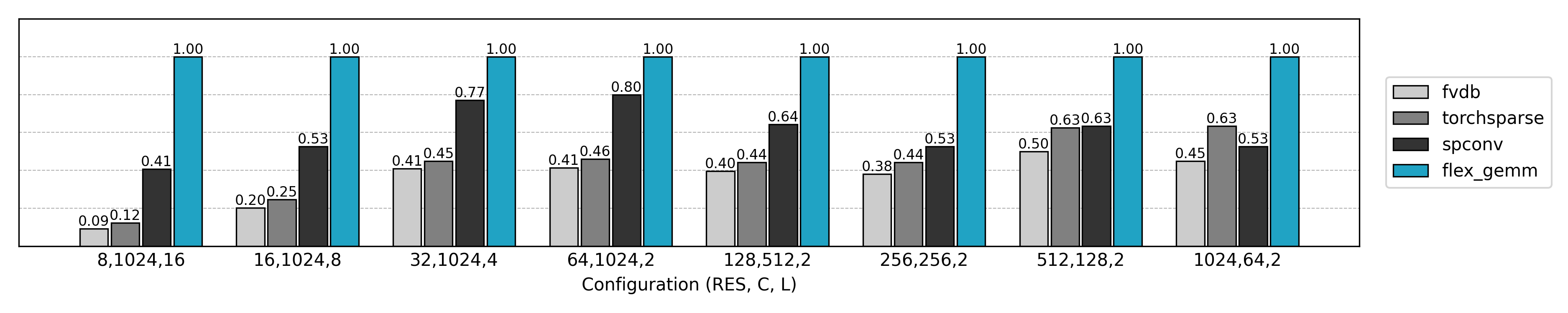
Performance Comparison

Compared to the final optimized implementation, the naive Explicit GEMM only achieves about 10% of the performance while consuming 10× more GPU memory. As the problem size grows, the Explicit GEMM algorithm degrades further. Clearly, new optimization methods are needed.

Skipping Expansion: Implicit GEMM

In the previous Explicit GEMM approach, we relied on PyTorch’s highly optimized matrix multiplication to implement convolution, so the computation itself was nearly optimal. However, explicitly constructing the expanded neighborhood matrix introduces two major issues:

First, the expanded matrix consumes a large amount of GPU memory. For an input feature tensor feats of shape [N, C] and kernel size [Kd, Kh, Kw], the expanded matrix has shape [N * V, C], where $V = Kd \cdot Kh \cdot Kw$. When the number of active voxels N or kernel size is large, memory usage grows explosively.

Second, and more importantly, there is significant global memory access overhead. In explicit expansion, each voxel’s neighborhood features are first written into a large expanded matrix, which must then be read again during the matrix multiplication. Given the scale of the expanded matrix, this repeated access severely impacts performance.

To address these issues, we can adopt Implicit GEMM: Instead of building the neighborhood-expanded matrix in advance, the gathering of input features by neighborhood index and the matrix multiplication are fused into a single GPU kernel. During computation, input features are accessed directly by index, and intermediate results are stored in shared memory, eliminating the need to construct the full expanded matrix in global memory. This not only dramatically reduces memory usage but also cuts down on global memory access, thereby improving sparse convolution efficiency on large-scale data.

Global Memory: Large-capacity GPU memory with high latency, accessible by all threads. Every read/write goes through the memory bus, suitable for storing inputs, outputs, and convolution weights.

Shared Memory: On-chip memory shared by threads within a block, much smaller in capacity but with very low latency. Ideal for caching intermediate results or small data tiles, reducing global memory accesses.

Triton to the Rescue

For such a fused operator, I chose Triton for the implementation.

Triton’s core design goal is to let developers write efficient GPU kernels with Python-like syntax, while automatically gaining many of the optimization capabilities usually only available in low-level CUDA programming. Compared to CUDA C++, it has several standout features:

Python-based syntax Triton kernels are written in Python and compiled JIT with the @triton.jit decorator. Compared to CUDA’s C++ syntax, Triton is much simpler and more intuitive, making it especially suited for research and rapid prototyping.
Program = one thread block In Triton, each kernel instance is called a program, roughly corresponding to a thread block in CUDA. You only need to think about how each program handles its data tile, without explicitly managing thread IDs and scheduling.
Block-level memory access Triton encourages working with rectangular tiles as the unit of loading and computation. With tl.load / tl.store, you explicitly control global memory access patterns, naturally supporting vectorized memory access.
Automatic register and shared memory management In CUDA, developers must explicitly declare and manage shared memory. Triton’s compiler, however, automatically places data into registers or shared memory depending on tile sizes and access patterns, achieving optimizations comparable to manual tuning.
Loop unrolling and pipelining Triton can analyze memory access and computation patterns, automatically unroll loops and schedule pipelines, hiding memory latency while maximizing compute utilization.
Auto-tuning With the @triton.autotune decorator, you can define multiple candidate configurations (e.g., tile size, thread count, pipeline depth). At runtime, Triton automatically benchmarks and picks the fastest configuration.

For Implicit GEMM, each active voxel’s neighborhood features must be loaded from global memory by index. If you follow a “load everything first, then compute” approach, the GPU often stalls while waiting for data. Triton’s compiler optimizes this automatically:

While one tile’s neighborhood features are being fetched from global memory, GPU threads can continue matrix multiplications on the previous tile’s data already in registers/shared memory, avoiding idle compute.
Triton generates coalesced memory access instructions, organizing neighborhood gather operations into batched, contiguous accesses to reduce bandwidth waste.
Intermediate feature tiles are cached in registers or shared memory, depending on which is faster for reuse.
Finally, with @triton.autotune, tile configurations are automatically optimized for different kernel sizes and input scales, ensuring load–compute overlap remains efficient across scenarios.

For readers interested in learning Triton kernel basics, see the official tutorials: Tutorials — Triton documentation

Forward Process

@triton.jit
def sparse_submanifold_conv_fwd_implicit_gemm_kernel(
    input,
    weight,
    bias,
    neighbor,
    output,
    # Tensor dimensions
    N, Ci, Co, V: tl.constexpr,
    # Meta-parameters
    B1: tl.constexpr,   # Block size for N dimension
    B2: tl.constexpr,   # Block size for Co dimension
    BK: tl.constexpr,   # Block size for K dimension (V * Ci)
    allow_tf32: tl.constexpr,  # Allow TF32 precision for matmuls
):
    """
    Sparse submanifold convolution forward kernel using implicit GEMM.
    
    Args:
        input (pointer): A pointer to the input tensor of shape (N, Ci)
        weight (pointer): A pointer to the weight tensor of shape (Co, V, Ci)
        bias (pointer): A pointer to the bias tensor of shape (Co)
        neighbor (pointer): A pointer to the neighbor tensor of shape (N, V)
        output (pointer): A pointer to the output tensor of shape (N, Co)
    """
    block_id = tl.program_id(axis=0)
    block_dim_co = tl.cdiv(Co, B2)
    block_id_co = block_id % block_dim_co
    block_id_n = block_id // block_dim_co
    
    # Create pointers for submatrices of A and B.
    num_k = tl.cdiv(Ci, BK)  # Number of blocks in K dimension
    offset_n = (block_id_n * B1 + tl.arange(0, B1)) % N         # (B1,)
    offset_co = (block_id_co * B2 + tl.arange(0, B2)) % Co      # (B2,)
    offset_k = tl.arange(0, BK)                                 # (BK,)
    
    # Create a block of the output matrix C.
    accumulator = tl.zeros((B1, B2), dtype=tl.float32)
    
    # Calculate pointers to weight matrix.
    weight_ptr = weight + (offset_co[None, :] * V * Ci + offset_k[:, None])     # (BK, B2)
    
    # Iterate along V*Ci dimension.
    for k in range(num_k * V):
        v = k // num_k
        bk = k % num_k
        # Calculate pointers to input matrix.
        neighbor_offset_n = tl.load(neighbor + offset_n * V + v)                                # (B1,)
        input_ptr = input + bk * BK + (neighbor_offset_n[:, None] * Ci + offset_k[None, :])     # (B1, BK)
        # Load the next block of input and weight.
        neigh_mask = neighbor_offset_n != 0xffffffff
        k_mask = offset_k < Ci - bk * BK
        input_block = tl.load(input_ptr, mask=neigh_mask[:, None] & k_mask[None, :], other=0.0)
        weight_block = tl.load(weight_ptr, mask=k_mask[:, None], other=0.0)
        # Accumulate along the K dimension.
        accumulator = tl.dot(input_block, weight_block, accumulator,
                             input_precision='tf32' if allow_tf32 else 'ieee')                  # (B1, B2)
        # Advance the pointers to the next Ci block.
        weight_ptr += min(BK, Ci - bk * BK)
    c = accumulator.to(input.type.element_ty)
            
    # add bias
    if bias is not None:
        bias_block = tl.load(bias + offset_co)
        c += bias_block[None, :]
                
    # Write back the block of the output matrix with masks.
    out_offset_n = block_id_n * B1 + tl.arange(0, B1)
    out_offset_co = block_id_co * B2 + tl.arange(0, B2)
    out_ptr = output + (out_offset_n[:, None] * Co + out_offset_co[None, :])
    out_mask = (out_offset_n[:, None] < N) & (out_offset_co[None, :] < Co)
    tl.store(out_ptr, c, mask=out_mask)

Next, let’s break down this Triton kernel step by step to see how it implements the Sparse Submanifold Convolution forward pass.

1. Overall Structure of the Kernel

@triton.jit
def sparse_submanifold_conv_fwd_implicit_gemm_kernel(
    input,
    weight,
    bias,
    neighbor,
    output,
    # Tensor dimensions
    N, Ci, Co, V: tl.constexpr,
    # Meta-parameters
    B1: tl.constexpr,   # Block size for N dimension
    B2: tl.constexpr,   # Block size for Co dimension
    BK: tl.constexpr,   # Block size for K dimension (V * Ci)
    allow_tf32: tl.constexpr,  # Allow TF32 precision for matmuls
):

This defines a Triton kernel:

input, weight, bias, neighbor, output are pointers to GPU global memory.
N, Ci, Co, V represent the number of input points, input channels, output channels, and neighborhood size.
B1, B2, BK define the tile sizes, i.e., the work unit of each kernel.
allow_tf32 enables TensorFloat32 precision for dot products.

This follows a tiled GEMM pattern: splitting the output matrix [N, Co] into tiles, each computed by one Triton program.

2. Program IDs and tile partitioning

    block_id = tl.program_id(axis=0)
    block_dim_co = tl.cdiv(Co, B2)
    block_id_co = block_id % block_dim_co
    block_id_n = block_id // block_dim_co

Each program (thread block) computes one output tile:

block_id_n: tile position along the N dimension
block_id_co: tile position along the Co dimension

So, each tile covers a [B1 × B2] region of the output.

3. Tile coordinate ranges

    offset_n = (block_id_n * B1 + tl.arange(0, B1)) % N
    offset_co = (block_id_co * B2 + tl.arange(0, B2)) % Co
    offset_k = tl.arange(0, BK)

offset_n: indices for this tile along N
offset_co: indices for this tile along Co
offset_k: indices along the Ci dimension for each block

Because shared memory is limited, we cannot load entire [B1, Ci] and [Ci, B2] submatrices at once, so we split them into [BK] chunks and accumulate results iteratively.

4. Accumulator initialization

    accumulator = tl.zeros((B1, B2), dtype=tl.float32)

Each tile maintains a [B1 × B2] accumulator initialized to zero. Results from multiple input/weight blocks are accumulated here.

5. Main loop: iterate over neighborhoods and channel blocks

    for k in range(num_k * V):
        v = k // num_k
        bk = k % num_k

This loop iterates over all neighborhoods (V) and input channel blocks (Ci // BK). The final result is built up block by block.

6. Implicit neighborhood feature loading

        neighbor_offset_n = tl.load(neighbor + offset_n * V + v)
        input_ptr = input + bk * BK + (neighbor_offset_n[:, None] * Ci + offset_k[None, :])
        input_block = tl.load(input_ptr, mask=neigh_mask[:, None] & k_mask[None, :], other=0.0)

neighbor stores neighbor indices for each voxel.
For each point offset_n, it retrieves the index of its v-th neighbor.
Using neighbor_offset_n, the corresponding input features are directly gathered.
A mask is applied: if a neighbor is missing (0xffffffff), load 0 instead.

This is the implicit expansion step: no [N*V, Ci] matrix is materialized in global memory. Instead, input features are fetched on demand per tile.

7. Weight loading and dot product

        weight_block = tl.load(weight_ptr, mask=k_mask[:, None], other=0.0)
        accumulator = tl.dot(input_block, weight_block, accumulator,
                             input_precision='tf32' if allow_tf32 else 'ieee')

weight_block: loads the relevant weight tile (BK × B2)
tl.dot: performs block-level matrix multiplication and accumulates into accumulator
FP32 accumulation ensures numerical stability

This is the core of Implicit GEMM.

8. Writing results back

    c = accumulator.to(input.type.element_ty)
    if bias is not None:
        bias_block = tl.load(bias + offset_co)
        c += bias_block[None, :]
    out_ptr = output + (out_offset_n[:, None] * Co + out_offset_co[None, :])
    tl.store(out_ptr, c, mask=out_mask)

Convert FP32 accumulators back to input dtype (e.g., FP16).
Add bias if provided.
Store results to global memory with masking to prevent out-of-bound writes.

Each tile writes back its slice of the output matrix, completing the sparse submanifold convolution forward pass.

Backward Process

The backward pass consists of computing gradients w.r.t. the input sparse tensor and the convolution weights. The implementation framework is similar to the forward kernel.

Gradients w.r.t. Input

As analyzed in the Explicit GEMM case, for submanifold convolution, we just flip the neighborhood indices and perform convolution of the output gradients with the kernel:

neighbor_offset_n = tl.load(neighbor + offset_n * V + V - 1 - v)

Gradients w.r.t. Weights

Multiply the output gradients with input features expanded by neighborhood indices:

mask = offset_k < N - k * BK
# Calculate pointers to input matrix.
input_offset_n = tl.load(neighbor_ptr, mask=mask[:, None], other=0xffffffff)            # (BK, BV)
input_ptr = input + (input_offset_n[:, :, None] * Ci + offset_ci[None, None, :])        # (BK, BV, BCi)
# Load the next block of input and weight.
grad_output_block = tl.load(grad_output_ptr, mask=mask[None, :], other=0.0)
input_block = tl.load(input_ptr, mask=input_offset_n[:, :, None] != 0xffffffff, other=0.0).reshape(BK, BV * BCi)
# Accumulate along the K dimension.
accumulator = tl.dot(grad_output_block, input_block, accumulator,
                    input_precision='tf32' if allow_tf32 else 'ieee')                  # (B1, B2)

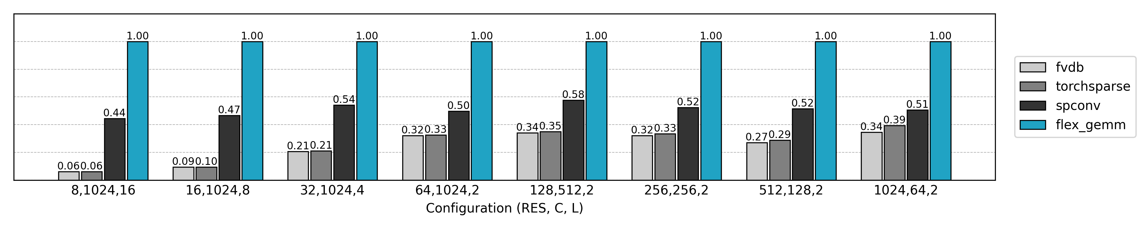
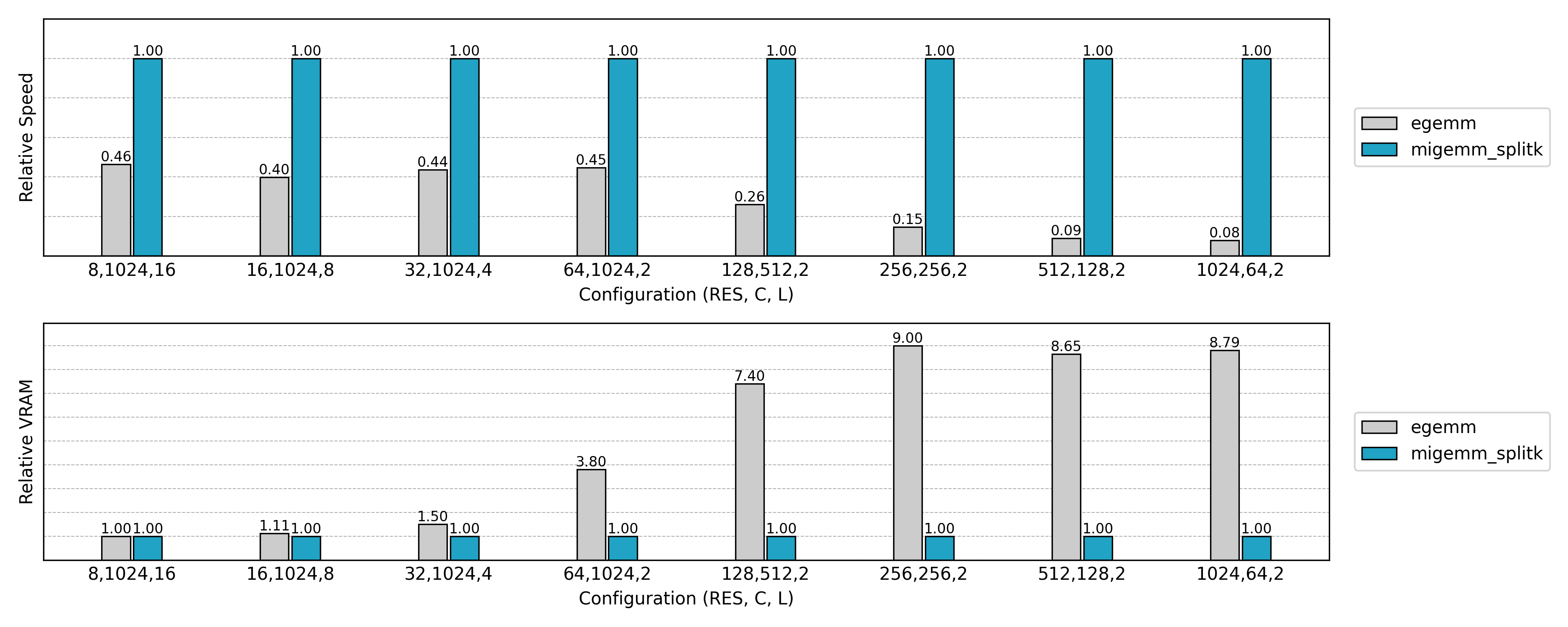
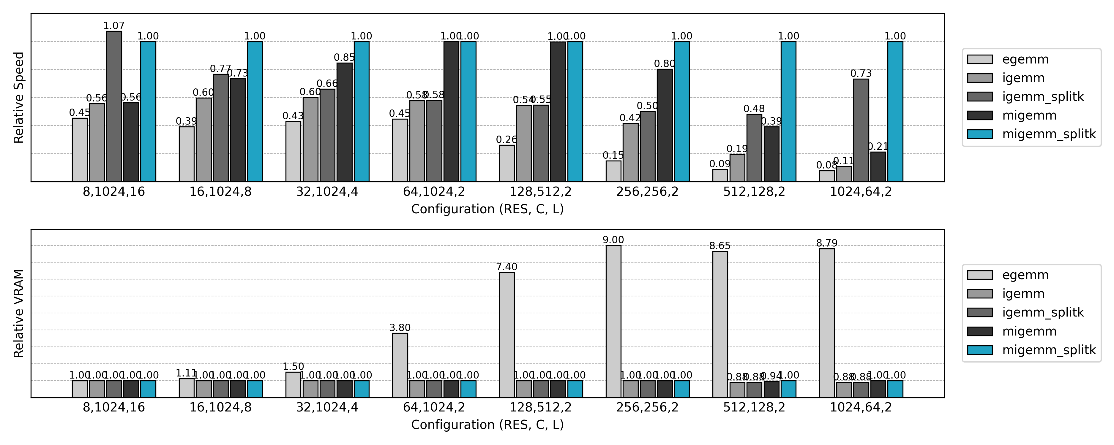
Performance Comparison

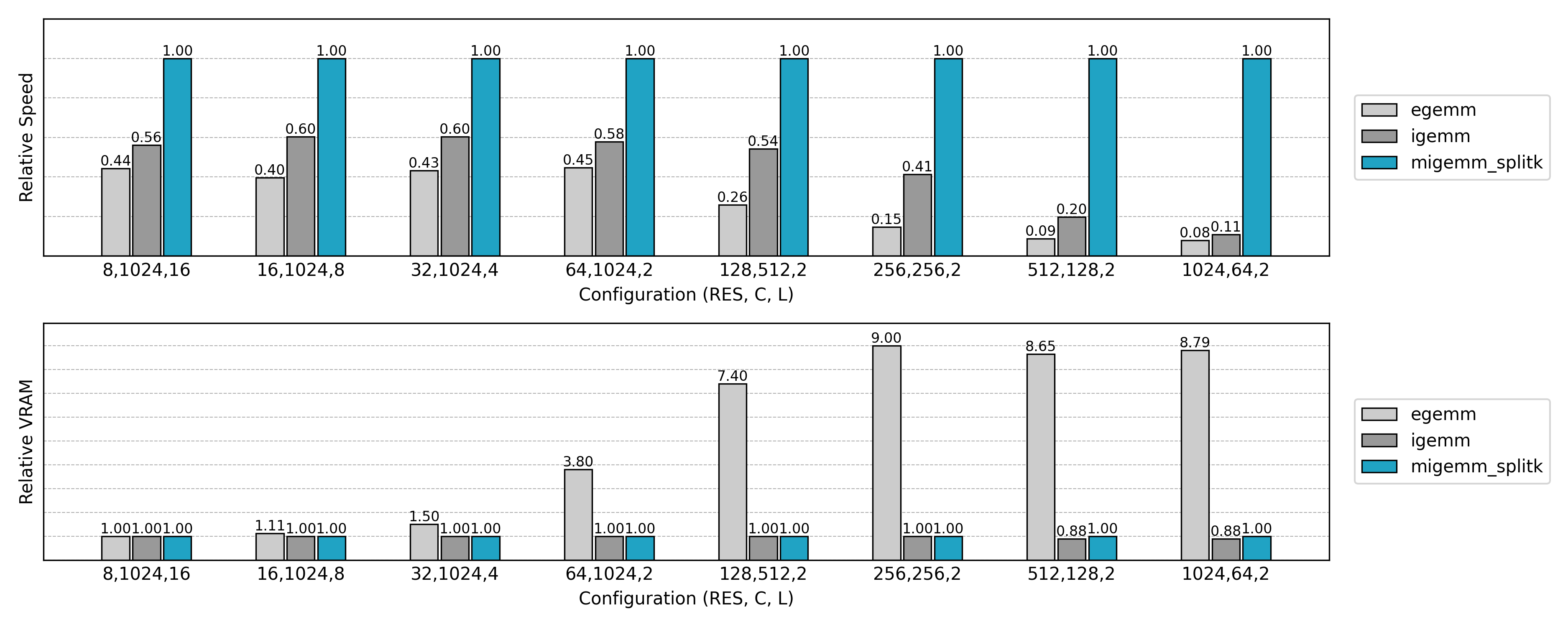
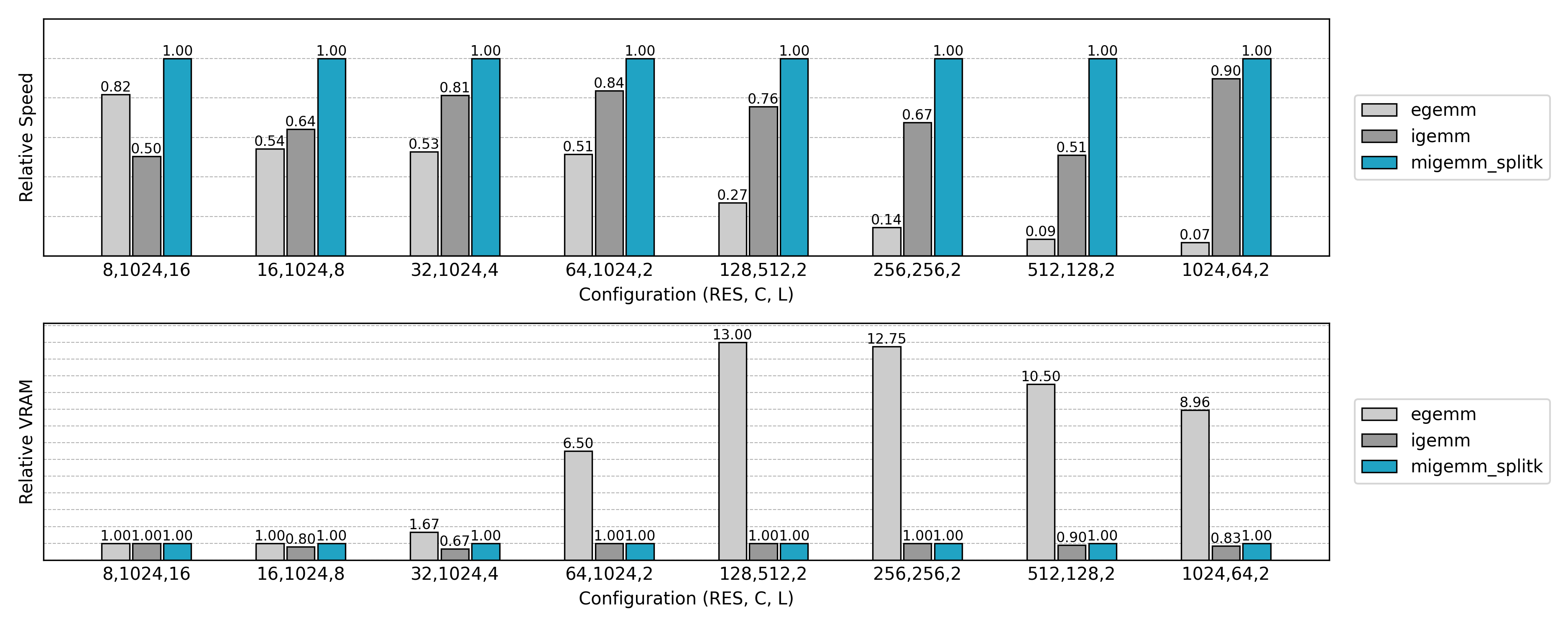
Compared to the earlier Explicit GEMM approach, the Implicit GEMM implementation achieves significant speedups and memory savings. However, some anomalies are observed:

For small spatial sizes with large channel counts, inference is slower than the naive method.
For large spatial sizes with small channel counts, training speed shows almost no improvement.

These results warrant further investigation.

Increasing Parallelism: Split K

Observing the previous speed tests, we can see that in some cases the runtime is significantly slower than the final implementation:

Small spatial size but large number of channels: forward pass and backward pass on input sparse tensor
Large spatial size but small number of channels: backward pass on convolution weights

These two scenarios share a common property: the GEMM K dimension (the accumulation dimension) is large, while the M or N dimensions (sources of parallelism) are insufficient.

Taking the forward pass as an example, the total computation is the product of three dimensions:

M dimension: corresponding to the number of input voxels N
N dimension: corresponding to the number of output channels Co
K dimension: corresponding to neighborhood size and input channels V * Ci

If M or N is small while K is large, a problem arises: GPU parallelism happens at the tile level, but if M and N are too small, the computation can only be divided into a few tiles (((M + B1 - 1) // B1) * ((N + B2 -1) // B2)). K is “serial accumulation” and cannot naturally provide parallelism. The result is underutilized GPU threads and idle SM units, leading to severe performance degradation.

Finer-Grained Parallelism

To solve this, Split K can be introduced:

Split the accumulation along the K dimension into multiple sub-tasks, each handling a portion of K.
Each sub-task can run as an independent kernel program in parallel, increasing overall parallelism.
Once all sub-tasks are complete, a reduction along M and N dimensions combines the results into the final output.

Formally:

\[\boldsymbol{C} = \boldsymbol{A} \times \boldsymbol{B} \quad (\boldsymbol{A}\in\mathbb{R}^{M \times K}, \boldsymbol{B}\in\mathbb{R}^{K \times N})\]

If K is split into S segments:

\[C = \sum_{s=0}^{S-1} A_{[:, K_s]} \times B_{[K_s, :]}\]

Each $A_{[:, K_s]} \times B_{[K_s, :]}$ can be computed in parallel.

Of course, Split K is not free:

It requires an extra reduction, accumulating partial sums into the final result.
This incurs additional global memory read/write overhead.
But in scenarios with insufficient parallelism, this cost is far less than the GPU idle time.

Therefore, Split K is generally enabled only when M or N is too small. In practice, autotune can automatically decide whether to enable it and select an appropriate S.

Code Implementation

For submanifold convolution forward pass, the backward pass can be modified similarly:

@triton.jit
def sparse_submanifold_conv_fwd_implicit_gemm_splitk_kernel(
    input,
    weight,
    bias,
    neighbor,
    output,
    # Tensor dimensions
    N, Ci, Co, V: tl.constexpr,
    # Meta-parameters
    B1: tl.constexpr,   # Block size for N dimension
    B2: tl.constexpr,   # Block size for Co dimension
    BK: tl.constexpr,   # Block size for K dimension (V * Ci)
    SPLITK: tl.constexpr,  # Split K dimension
    allow_tf32: tl.constexpr,  # Allow TF32 precision for matmuls
):
    """
    Sparse submanifold convolution forward kernel using implicit GEMM with split K dimension.
    
    Args:
        input (pointer): A pointer to the input tensor of shape (N, Ci)
        weight (pointer): A pointer to the weight tensor of shape (Co, V, Ci)
        bias (pointer): A pointer to the bias tensor of shape (Co)
        neighbor (pointer): A pointer to the neighbor tensor of shape (N, V)
        output (pointer): A pointer to the output tensor of shape (N, Co)
    """
    block_id_k = tl.program_id(axis=1)  # SplitK dimension
    block_id = tl.program_id(axis=0)
    block_dim_co = tl.cdiv(Co, B2)
    block_id_co = block_id % block_dim_co
    block_id_n = block_id // block_dim_co
    
    # Create pointers for submatrices of A and B.
    num_k = tl.cdiv(Ci, BK)  # Number of blocks in K dimension
    k_start = tl.cdiv(num_k * V * block_id_k, SPLITK)
    k_end = tl.cdiv(num_k * V * (block_id_k + 1), SPLITK)
    offset_n = (block_id_n * B1 + tl.arange(0, B1)) % N         # (B1,)
    offset_co = (block_id_co * B2 + tl.arange(0, B2)) % Co      # (B2,)
    offset_k = tl.arange(0, BK)                                 # (BK,)
    
    # Create a block of the output matrix C.
    accumulator = tl.zeros((B1, B2), dtype=tl.float32)
    
    # Calculate pointers to weight matrix.
    weight_ptr = weight + k_start * BK + (offset_co[None, :] * V * Ci + offset_k[:, None])     # (BK, B2)
    
    # Iterate along V*Ci dimension.
    for k in range(k_start, k_end):
        v = k // num_k
        bk = k % num_k
        # Calculate pointers to input matrix.
        neighbor_offset_n = tl.load(neighbor + offset_n * V + v)                                # (B1,)
        input_ptr = input + bk * BK + (neighbor_offset_n[:, None] * Ci + offset_k[None, :])     # (B1, BK)
        # Load the next block of input and weight.
        neigh_mask = neighbor_offset_n != 0xffffffff
        k_mask = offset_k < Ci - bk * BK
        input_block = tl.load(input_ptr, mask=neigh_mask[:, None] & k_mask[None, :], other=0.0)
        weight_block = tl.load(weight_ptr, mask=k_mask[:, None], other=0.0)
        # Accumulate along the K dimension.
        accumulator = tl.dot(input_block, weight_block, accumulator,
                             input_precision='tf32' if allow_tf32 else 'ieee')                  # (B1, B2)
        # Advance the pointers to the next Ci block.
        weight_ptr += min(BK, Ci - bk * BK)
            
    # add bias
    if bias is not None and block_id_k == 0:
        bias_block = tl.load(bias + offset_co)
        accumulator += bias_block[None, :]
                
    # Write back the block of the output matrix with masks.
    out_offset_n = block_id_n * B1 + tl.arange(0, B1)
    out_offset_co = block_id_co * B2 + tl.arange(0, B2)
    out_ptr = output + block_id_k * N * Co + (out_offset_n[:, None] * Co + out_offset_co[None, :])
    out_mask = (out_offset_n[:, None] < N) & (out_offset_co[None, :] < Co)
    tl.store(out_ptr, accumulator, mask=out_mask)

The above kernel is similar to the Implicit GEMM implementation, but the core difference is how the K dimension is handled. Let’s highlight the key differences.

1. Additional program_id dimension

block_id_k = tl.program_id(axis=1)  # SplitK dimension
block_id = tl.program_id(axis=0)

In ordinary Implicit GEMM, each program is distinguished only by axis=0 for (N, Co) tiles. In SplitK, we additionally introduce axis=1, which represents the segment of the K dimension. This allows each (N, Co) tile to be computed by multiple programs in parallel, with each program handling only a portion of the K dimension.

2. Determining K range

num_k = tl.cdiv(Ci, BK)
k_start = tl.cdiv(num_k * V * block_id_k, SPLITK)
k_end = tl.cdiv(num_k * V * (block_id_k + 1), SPLITK)

Ordinary Implicit GEMM traverses the entire K = V * Ci. SplitK divides it into SPLITK segments:

k_start and k_end indicate the K range assigned to the current block_id_k.
This ensures that even if N or Co is small, parallelism can be increased by splitting K.

3. Reduced loop range

for k in range(k_start, k_end):
    ...

Compared to Implicit GEMM, which traverses all num_k * V, this loop only covers [k_start, k_end), with weight pointers starting at k_start. This is the key of SplitK: each program computes only a portion of the K contribution.

4. Bias addition logic change

if bias is not None and block_id_k == 0:
    bias_block = tl.load(bias + offset_co)
    accumulator += bias_block[None, :]

In Implicit GEMM, each (N, Co) tile adds bias directly. In SplitK, the same (N, Co) tile may be computed by multiple programs. If bias is added in every segment, it would be counted multiple times. Hence, the addition is restricted to block_id_k == 0 only.

5. Writing output to segmented buffer

out_ptr = output + block_id_k * N * Co + (out_offset_n[:, None] * Co + out_offset_co[None, :])

In Implicit GEMM, the result is written directly to [N, Co]. In SplitK, each block_id_k writes to a separate segment (the block_id_k-th segment). The final output tensor shape is effectively [SPLITK, N, Co] and requires an external reduction (sum) to obtain the true [N, Co].

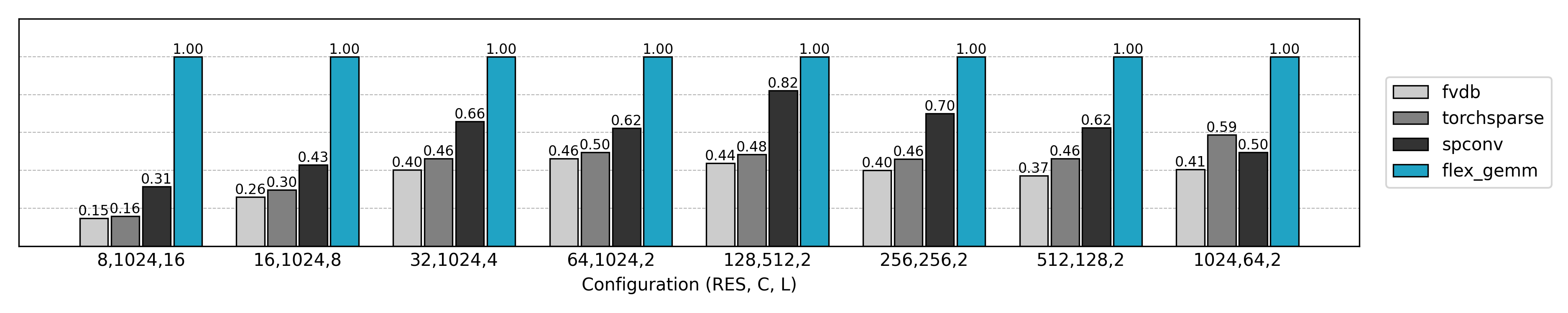
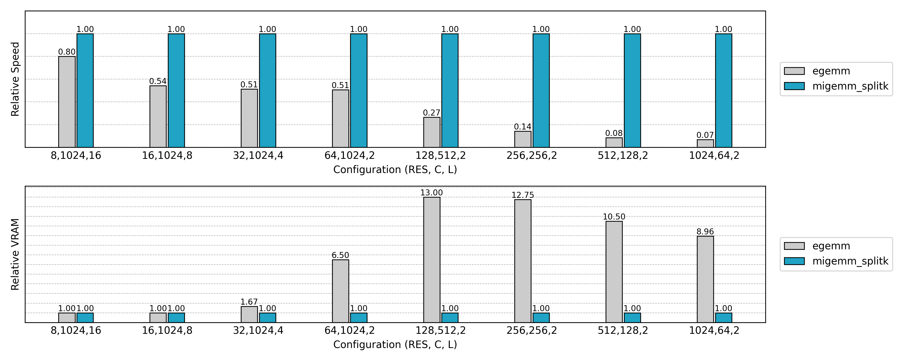
Performance Comparison

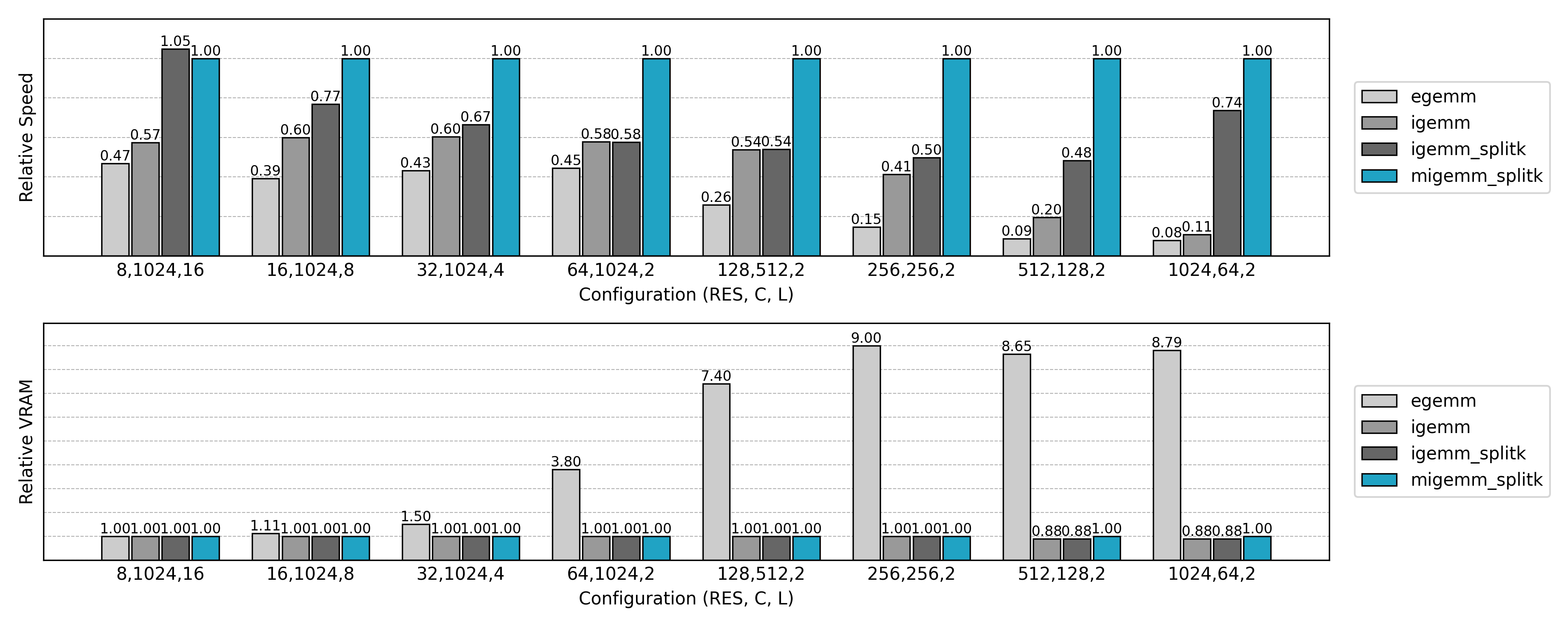
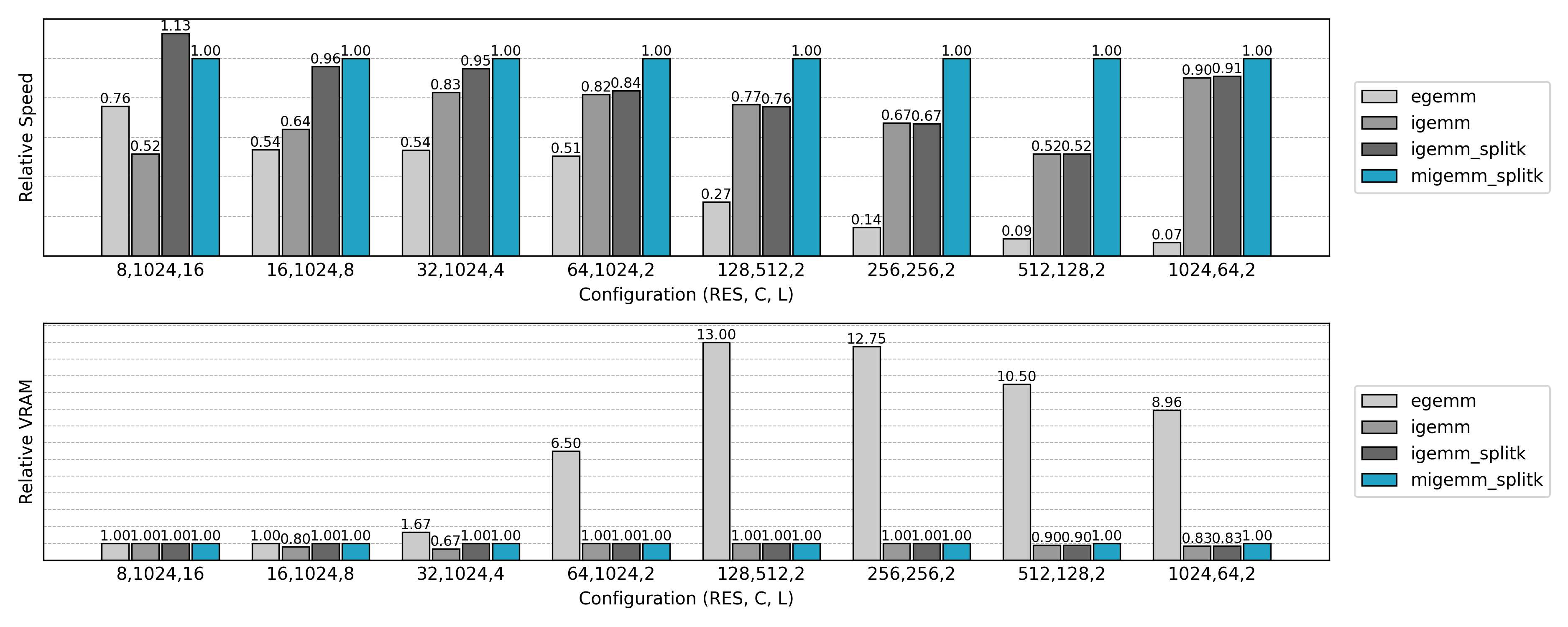
Compared to the non-Split K version, GPU utilization is significantly improved in small N or small Co scenarios.

SIMD-Aware Scheduling: Masked Implicit GEMM

In sparse convolution, many active voxels have some neighborhood positions that are actually “empty” (i.e., no valid neighbor, represented by 0xffffffff in the code). If we still traverse all V neighborhood positions, a large amount of unnecessary loading and multiply-add operations will be performed on these “empty” positions, wasting memory bandwidth and compute resources. This leads to the next optimization goal — skip (or minimize) computation on these empty neighborhoods, focusing compute resources on the neighbors that actually exist, resulting in significant acceleration in highly sparse scenarios.

On the CPU, this optimization is simple: when traversing neighbors, just continue on invalid indices.

On GPUs, due to the Single Instruction Multiple Data (SIMD) execution model, threads within a warp must follow the same execution path. Only when all threads in a warp have an empty neighbor at a certain position can we skip memory access and computation for that position. If different threads branch differently at some neighbor positions (some have neighbors, some do not), the GPU will execute as if the neighbor exists for all threads, yielding no speedup.

Single Instruction Multiple Data (SIMD) On a GPU, a warp (typically 32 threads) can execute only a single instruction at a time, operating on different data. If threads in a warp encounter a conditional branch (some taking if, others taking else), the GPU executes both branches sequentially and merges the results — this is called warp divergence. Therefore, in efficient GPU kernels, it is crucial to ensure that all threads in a block execute the same instructions to maximize efficiency.

Better task assignment

This raises a key question: how to assign neighborhood masks to compute blocks more efficiently?

Suppose we have many active voxels, each with a neighborhood mask represented as a binary vector (1 = neighbor exists, 0 = empty). If we assign these masks randomly to blocks, some blocks may contain threads with highly different neighborhood patterns:

Some threads have 1 at a position, requiring memory access and multiply-add.
Other threads have 0 at the same position, which actually does not need computation.

As a result, the entire warp must still execute the computation, and threads corresponding to empty neighbors are forced to “follow along,” lowering efficiency.

In other words, the union of all neighbor masks within a block determines how many neighbor positions the block must process. The optimization goal can be abstracted as:

Group all neighborhood masks into blocks of fixed size (block size), minimizing the sum of the union of masks within each block.

From an algorithmic perspective, this is a hard partitioning problem, but heuristic methods can be used to approximate the optimal solution.

Gray code ordering

A simple yet effective approach in practice is Gray Code Ordering.

Gray codes have the property that adjacent codes differ by only one bit. This means that if we reorder voxel neighborhood masks according to Gray code order, adjacent elements will have similar binary patterns.

Using this property:

First, map all voxel neighborhood masks to Gray code values.
Sort the voxels according to Gray code order.
Then, divide them into blocks of fixed size sequentially.

The benefit of this grouping is natural: masks within a block are “close” in bit space, so differences are concentrated in a few bit positions. As a result, the threads in the same block have more consistent execution logic, reducing wasted computation and minimizing unnecessary memory access and multiply-add operations on the GPU.

Neighborhood cache information

The Masked Implicit GEMM kernel relies on the following cached information:

neighbor_map: same as in Explicit/Implicit GEMM, recording the mapping between voxels and their neighbors; empty positions are marked as 0xffffffff.
sorted_idx: active voxel indices reordered according to Gray code.
valid_kernel_{block_size} and valid_kernel_seg_{block_size}: for a given block size, each block’s set of valid neighbors. Positions where all threads are empty are excluded, forming a variable-length array for efficient kernel indexing.
valid_signal_i / valid_signal_o and valid_signal_seg: record the valid input/output tensor indices corresponding to each neighbor position, used in backward propagation of convolution weight gradients.

Overall, these cached data can be understood as an execution plan constructed before the operator runs. Using this plan, the Masked Implicit GEMM kernel can remain SIMD-friendly while skipping computation on empty neighborhoods, achieving significant speedup on highly sparse inputs.

The CUDA implementation is relatively straightforward. Readers can refer to flex_gemm\kernels\cuda\spconv\neighbor_map.cu (L255) for code and flex_gemm\ops\spconv\submanifold_conv3d.py (L9) for Python interfaces.

Forward pass

Using the reorganized execution plan and cached neighborhood info, the Triton implementation of the Masked Implicit GEMM forward pass for submanifold convolution is:

@triton.jit
def sparse_submanifold_conv_fwd_masked_implicit_gemm_splitk_kernel(
    input,
    weight,
    bias,
    neighbor,
    sorted_idx,
    output,
    # Tensor dimensions
    N, Ci, Co, V: tl.constexpr,
    # Meta-parameters
    B1: tl.constexpr,   # Block size for N dimension
    B2: tl.constexpr,   # Block size for Co dimension
    BK: tl.constexpr,   # Block size for K dimension (V * Ci)
    SPLITK: tl.constexpr,  # Split K dimension into multiple sub-dimensions
    allow_tf32: tl.constexpr,  # Allow TF32 precision for matmuls
    # Huristic parameters
    valid_kernel,
    valid_kernel_seg,
):
    """
    Sparse submanifold convolution forward kernel using masked implicit GEMM split-k.
    
    Args:
        input (pointer): A pointer to the input tensor of shape (N, Ci)
        weight (pointer): A pointer to the weight tensor of shape (Co, V, Ci)
        bias (pointer): A pointer to the bias tensor of shape (Co)
        neighbor (pointer): A pointer to the neighbor tensor of shape (N, V)
        sorted_idx (pointer): A pointer to the sorted index tensor of shape (N)
        valid_kernel (pointer): A pointer to the valid neighbor index tensor of shape (L)
        valid_kernel_seg (pointer): A pointer to the valid neighbor index segment tensor of shape (BLOCK_N + 1)
        output (pointer): A pointer to the output tensor of shape (N, Co)
    """
    block_id_k = tl.program_id(axis=1)  # SplitK dimension
    block_id = tl.program_id(axis=0)
    block_dim_co = tl.cdiv(Co, B2)
    block_id_co = block_id % block_dim_co
    block_id_n = block_id // block_dim_co
    
    # Create pointers for submatrices of A and B.
    num_k = tl.cdiv(Ci, BK)  # Number of blocks in K dimension
    valid_kernel_start = tl.load(valid_kernel_seg + block_id_n)
    valid_kernel_seglen = tl.load(valid_kernel_seg + block_id_n + 1) - valid_kernel_start
    k_start = tl.cdiv(num_k * valid_kernel_seglen * block_id_k, SPLITK)
    k_end = tl.cdiv(num_k * valid_kernel_seglen * (block_id_k + 1), SPLITK)
    offset_n = block_id_n * B1 + tl.arange(0, B1)
    n_mask = offset_n < N
    offset_sorted_n = tl.load(sorted_idx + offset_n, mask=n_mask, other=0)  # (B1,)
    offset_co = (block_id_co * B2 + tl.arange(0, B2)) % Co                  # (B2,)
    offset_k = tl.arange(0, BK)                                             # (BK,)
    
    # Create a block of the output matrix C.
    accumulator = tl.zeros((B1, B2), dtype=tl.float32)
    
    # Iterate along V*Ci dimension.
    for k in range(k_start, k_end):
        v = k // num_k
        bk = k % num_k
        v = tl.load(valid_kernel + valid_kernel_start + v)
        # Calculate pointers to input matrix.
        neighbor_offset_n = tl.load(neighbor + offset_sorted_n * V + v)                             # (B1,)
        input_ptr = input + bk * BK + (neighbor_offset_n[:, None] * Ci + offset_k[None, :])         # (B1, BK)
        # Calculate pointers to weight matrix.
        weight_ptr = weight + v * Ci + bk * BK + (offset_co[None, :] * V * Ci + offset_k[:, None])  # (BK, B2)
        # Load the next block of input and weight.
        neigh_mask = neighbor_offset_n != 0xffffffff
        k_mask = offset_k < Ci - bk * BK
        input_block = tl.load(input_ptr, mask=neigh_mask[:, None] & k_mask[None, :], other=0.0)
        weight_block = tl.load(weight_ptr, mask=k_mask[:, None], other=0.0)
        # Accumulate along the K dimension.
        accumulator = tl.dot(input_block, weight_block, accumulator,
                             input_precision='tf32' if allow_tf32 else 'ieee')                      # (B1, B2)
            
    # add bias
    if bias is not None and block_id_k == 0:
        bias_block = tl.load(bias + offset_co)
        accumulator += bias_block[None, :]
                
    # Write back the block of the output matrix with masks.
    out_offset_n = offset_sorted_n
    out_offset_co = block_id_co * B2 + tl.arange(0, B2)
    out_ptr = output + block_id_k * N * Co + (out_offset_n[:, None] * Co + out_offset_co[None, :])
    out_mask = n_mask[:, None] & (out_offset_co[None, :] < Co)
    tl.store(out_ptr, accumulator, mask=out_mask)

Next, let’s go through the optimized Masked Implicit GEMM implementation combined with Split K step by step:

1. Block ID and dimension division

block_id_k = tl.program_id(axis=1)  # SplitK dimension
block_id = tl.program_id(axis=0)
block_dim_co = tl.cdiv(Co, B2)
block_id_co = block_id % block_dim_co
block_id_n = block_id // block_dim_co

Similar to the ordinary SplitK version:

block_id_n controls the input points block.
block_id_co controls the output channels block.
block_id_k controls the K dimension split.

2. Valid neighborhood range

valid_kernel_start = tl.load(valid_kernel_seg + block_id_n)
valid_kernel_seglen = tl.load(valid_kernel_seg + block_id_n + 1) - valid_kernel_start
k_start = tl.cdiv(num_k * valid_kernel_seglen * block_id_k, SPLITK)
k_end = tl.cdiv(num_k * valid_kernel_seglen * (block_id_k + 1), SPLITK)

This is the key difference of the Masked algorithm:

Each input point block_id_n has a valid kernel range obtained via valid_kernel_seg.
The loop range k_start ~ k_end no longer covers the full V * Ci, but only valid kernel positions.

Compared to the ordinary version, this reduces many empty iterations.

3. Neighbor index & input block loading

v = tl.load(valid_kernel + valid_kernel_start + v)
neighbor_offset_n = tl.load(neighbor + offset_sorted_n * V + v)    # (B1,)
input_ptr = input + bk * BK + (neighbor_offset_n[:, None] * Ci + offset_k[None, :])

Here, v comes from valid_kernel (valid kernel indices), not the original full range 0 ~ V-1. Input access follows the Gray code order to reduce unnecessary neighbors and memory/computation redundancy.

Also, neigh_mask = neighbor_offset_n != 0xffffffff masks out invalid points.

4. Weight block loading & multiply-accumulate

weight_ptr = weight + v * Ci + bk * BK + (offset_co[None, :] * V * Ci + offset_k[:, None])
input_block = tl.load(input_ptr, mask=neigh_mask[:, None] & k_mask[None, :], other=0.0)
weight_block = tl.load(weight_ptr, mask=k_mask[:, None], other=0.0)
accumulator = tl.dot(input_block, weight_block, accumulator,
                     input_precision='tf32' if allow_tf32 else 'ieee')

Similar to ordinary SplitK:

tl.dot performs matrix multiply-accumulate.
mask ensures no out-of-bound accesses.

Difference:

Weights are taken only for valid_kernel positions, not the full V.

5. Write back results

out_offset_n = offset_sorted_n
out_offset_co = block_id_co * B2 + tl.arange(0, B2)
out_ptr = output + block_id_k * N * Co + (out_offset_n[:, None] * Co + out_offset_co[None, :])
tl.store(out_ptr, accumulator, mask=out_mask)

The write-back process is the same as ordinary SplitK. If SPLITK > 1, an external reduction kernel sums results from different block_id_k for the same output block.

Backward pass

The forward pass skips empty neighborhoods using valid neighborhood indices, reducing unnecessary computation. The backward pass follows a similar logic:

Gradient w.r.t input features: Simply convolve the output gradient with flipped weights, loading weights in reverse:

weight_ptr = weight + (((offset_k[:, None] + bk * BK) * V + V - 1 - v) * Ci + offset_ci[None, :])

Gradient w.r.t convolution weights: Use cached valid_signal_i/o to load input features and output gradients, accumulate via matrix multiply, and optionally apply Split K optimization.

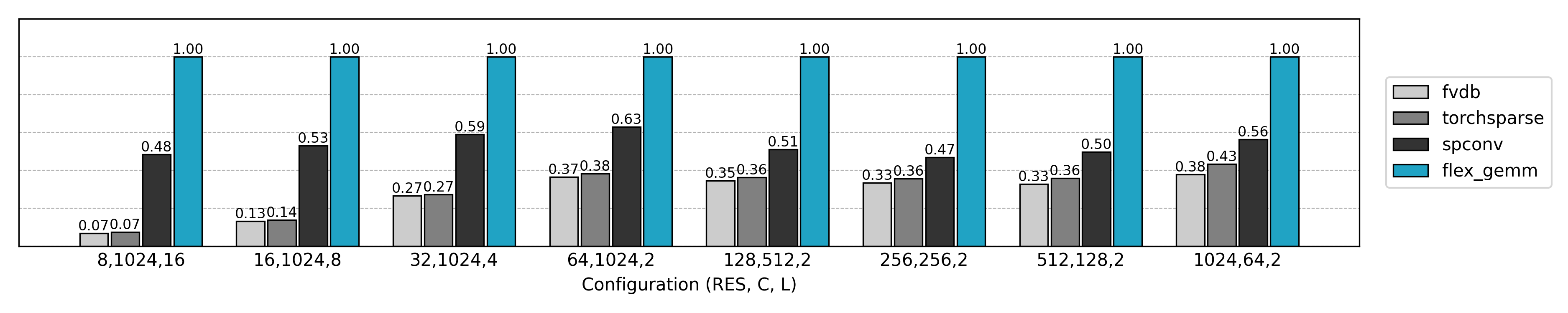
Performance comparison

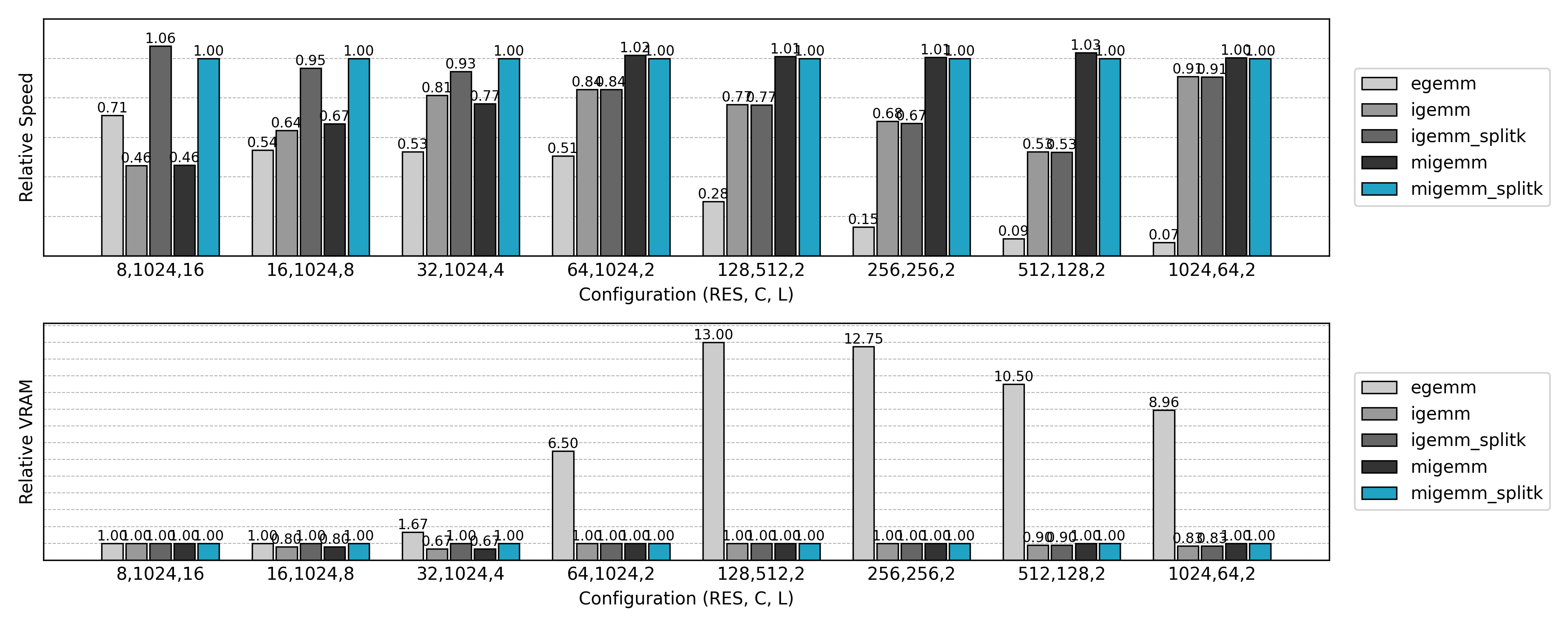
Speed tests show that Masked Implicit GEMM often improves performance by 20%–40% over ordinary Implicit GEMM.

Summary

The efficient implementation of sparse convolutions in FlexGEMM has undergone a continuous evolution.

At the foundation of everything lies the hash table, used for neighborhood queries to quickly establish the adjacency relationships required for convolutions in sparse scenarios.

The initial approach transformed convolution into standard matrix multiplication. Explicit GEMM, through an im2col-like unfolding, maximized the use of existing high-performance matrix libraries. However, due to extensive global memory usage, its efficiency and memory footprint were less than ideal.

To alleviate this, Implicit GEMM was proposed: it avoids explicit unfolding and computes on-demand within the kernel, reducing memory usage. Yet, it still suffers from warp divergence in parallel scheduling, wasting computation due to inconsistent neighbor access patterns across threads.

To further improve hardware utilization, Masked Implicit GEMM introduces a masking mechanism, skipping invalid computations and optimizing thread scheduling, achieving better overall performance.

An orthogonal improvement, SplitK, divides the accumulation dimension in matrix multiplication into multiple sub-tasks, which are then reduced at the end. This significantly enhances parallelism and execution efficiency in certain scenarios.

This evolution clearly illustrates the gradual transition of sparse convolutions from “feasible” to “efficient”: each generation of methods addresses the shortcomings of the previous one. Ultimately, the combination of Masked Implicit GEMM with SplitK usually delivers the best performance. Meanwhile, earlier Explicit and Implicit implementations remain valuable—they fully document the thought process and provide a reference for future research and optimization.

In our 3D generative model Trellis.2, FlexGEMM has already become a core operator. It enables high-resolution experiments even with limited hardware, while ensuring efficient and stable inference.

FlexGEMM is fully open-sourced, and we look forward to the community further extending these ideas in practice, driving continuous optimization of sparse convolution operators.

Preface

Starting from Naive Convolutions

Fetching Local Neighborhoods

Hash Tables on GPU

Insert

Lookup

Inserting Sparse Tensor Coordinates

Querying Neighborhood Indices

1. Thread assignment

2. Compute kernel center offset

3. Boundary check

4. Hash table lookup

5. Update neighbor map

Naive Implementation: Explicit GEMM

Neighborhood Cache

Forward Process

Backward Process

Performance Comparison

Skipping Expansion: Implicit GEMM

Triton to the Rescue

Forward Process

1. Overall Structure of the Kernel

2. Program IDs and tile partitioning

3. Tile coordinate ranges

4. Accumulator initialization

5. Main loop: iterate over neighborhoods and channel blocks

6. Implicit neighborhood feature loading

7. Weight loading and dot product

8. Writing results back

Backward Process

Gradients w.r.t. Input

Gradients w.r.t. Weights

Performance Comparison

Increasing Parallelism: Split K

Finer-Grained Parallelism

Code Implementation

1. Additional program_id dimension

2. Determining K range

3. Reduced loop range

4. Bias addition logic change

5. Writing output to segmented buffer

Performance Comparison

SIMD-Aware Scheduling: Masked Implicit GEMM

Better task assignment

Gray code ordering

Neighborhood cache information

Forward pass

1. Block ID and dimension division

2. Valid neighborhood range

3. Neighbor index & input block loading

4. Weight block loading & multiply-accumulate

5. Write back results

Backward pass

Performance comparison

Summary

References